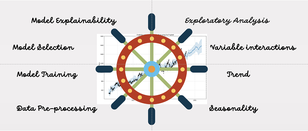
 Time Series Modelling flywheel
Authors: Debdut Banerjee, Ritesh Singh, Rishika Dasani, Mahashweta G
Introduction
Within Walmart, forecasting volume (cases, pallets, trailers, labor) is an integral part of our day-to-day operations to enable smooth flow of items from our suppliers to stores and our customers. Reliable forecasts are needed to minimize costs accrued due to over-forecasting or under-forecasting and in accordance with Walmart’s philosophy of EDLP (Every Day Low Price) and EDLC (Every Day Low Cost).
We often work with thousands of time series, having different patterns and behavior, which arise due to the complexities of our Supply chain network. Items have different seasonality, replenishment velocity and flow between a complex set of nodes in the supply chain consisting of consolidation centers, distribution centers, fulfilment centers, Import/Fashion DCs before they reach Walmart stores and finally to our customers. Walmart’s supply chain is also dynamic —there are new buildings which we need to forecast for, alignments are dynamic between suppliers, consolidation centers, DCs and stores, unpredictable weather and events like Covid 19, promotions and campaigns which make forecasting different volumes challenging.
In this process, as data scientists, we work with business and operations teams to enable them to leverage the forecasts to make more informed and data-driven planning decisions. We not only need to generate forecasts with high accuracy but also provide a framework to understand the factors that influence them. In this blog, we discuss an end-to-end framework that automates the forecasting process with commonly used data pre-processing techniques, wide selection of time-based feature generation pipelines, automatic model selection combining Time series, Linear and Tree based methods using different error metrics and forecast explainability framework.
Why is automatic model selection needed?
Traditional forecasting model development involves back-testing using different time series algorithms with each algorithm tuned on different hyperparameter settings. The problem with this approach is if the time series changes its pattern, a model which was picked up based on historical back-testing may no longer be a good fit for the data in production environment. Therefore, in production systems, continuous back-testing is needed to capture any data drift to the series and forecast using the best fit model automatically.

Also, as we can see from the above images, we have different kinds of time series having different patterns, making it necessary to consider multiple models rather than using a one-fits-all approach. The model which generates better predictions in the recent validation window gets selected rather than model selection based on intuition or back-testing performance in history.
 The Autotuning Forecast Framework
Data Pre-processing
The data pre-processing steps incorporated in the Autotuning Framework are:
- Autodetecting frequency of the time series: Autotuning Framework automatically detects the frequency of the series if the time series class is initiated with ‘auto’ frequency detection. The function requires a minimum of 8 data instances to infer the frequency of the series. If user can also provide the frequency of the time series to the ‘freq’ parameter when initiating the series if auto-detection of the frequency is not required.
- Missing data imputation: Since the presence of NaN values and missing time stamps in the data can lead to problems in some models, the time series needs to be first made continuous which can be done using the make_ts_cont method. This module enables the imputation of missing values in the time series using various approaches like:
- Rolling statistic (mean, median, minimum, maximum) imputation for given window length
- Day of the week imputation where the missing data is imputed with the average/median of previous collected at the same day of the week within the rolling window. This is only for daily time series.
The arguments the user can provide are the preferred method of imputation, rolling window length. The default imputation is 0. - Outlier treatment: This module enables the detection and subsequent imputation of outlier values.
Identification - The time series is first decomposed into trend, seasonal and residual components using additive or multiplicative decomposition, the residuals are then normalized and outliers detected using the IQR approach.
The outlier bounds are given below. Any residuals lying outside these bounds are identified as outliers.
[Q1- threshold_multiplierIQR, Q3+ threshold_multiplierIQR].
Imputation: The identified outliers are imputed with the imputation method of choice. The possible options for imputation are the same as those for missing value imputation.
The arguments the user can provide are the preferred method time series decomposition, the threshold multiplier, the preferred method of imputation, rolling window length. The user can also identify and treat outliers in other independent variables in addition to the target variable. This method requires presence of at least 2 cycles of data. - Data Drift detection: This module enables the user to visualize any drift/changepoints in the time series data. The changepoints are detected using an algorithm called PELT (Pruned Exact Linear Time). The intuition behind PELT is that a time step is detected as a change point only if it reduces the segmentation cost by more than the penalty value. The choice of penalty value can largely impact the changepoints detected for which CROPS (Changepoints for a Range of Penalties) is used that helps optimize the choice of penalty value.
The user needs to provide as an input the following:
- min_seg_length: the minimum length of a continuous segment
- jump_param: the number time steps between changepoints
- smaller_diff_detected: Minimum absolute difference between medians of 2 segments for the changepoint to be considered valid
- var: Variable for which changepoint detection is desired. Default value is ‘y’
Feature Engineering
Autotuning framework has a feature engineering module that allows the user to create certain families of features from the independent and dependent variables. The user can create the following families of features:
- Lagged features: Autotuning framework allows the user to create lag-based features of the dependent variable or independent variables once the user provides a dictionary specifying the features to be lagged and lag horizon required as values.
- Volume based features: If the time series is of weekly frequency, autotuning framework can create certain volume-based features that compute volume observed in the same weeks during past few years.
For example,
- Type “Lx00”, creates a feature which is the average volume in last x years of same week, i.e., if we are at Week 202412 and x=2, then volume of Week 202212 and 202312 is the new feature based on measure type.
- Type “Lxyz”, creates a feature which is the average volume in last x years of same week and y weeks backward and z weeks forward, i.e., if we are at Week 202412 and (x=3, y = 3, z = 3), then then value of the following 21 (3*(3+3+1)) weeks is the final feature based on measure type
Year 1 : 202109, 202110, 202111, 202112, 202113, 202114, 202115,
Year 2 : 202209, 202210, 202211, 202212, 202213, 202214, 202215,
Year 3 : 202309, 202310, 202311, 202312, 202313, 202314, 202315
The user needs to pass the type of feature and measure type as an argument so that all these x*(y+z+1) volume values can be aggregated into one valuue. - Rolling mean-based features: Autotuning framework allows the user to create rolling mean features of the dependent variable or independent variables once the user provides a dictionary specifying the features and the horizon for which the rolling mean is to be computed. Rolling mean computation is done in a way that till the refresh date actual values of the variable is used and after the refresh date a moving average forecast is used in place of actuals. Rolling mean is then computed using these “updated actuals” field.
During back-testing when a range of validation dates before the refresh dates are tried, computation of rolling mean is done using the validation dates as refresh dates to ensure there is no leakage of future information in the model selection exercise.
The user needs to pass the name of the rolling mean feature in the regressor dictionary to autotuning class. The rolling mean features should be named as:
‘root variable name+’rolling_mean’+rolling_window_length’.
For example, if we want to compute rolling mean of a variable y for window length 3 and 6, then they need to be passed as [‘y_rolling_mean_3’, ‘y_rolling_mean_6’] - One-hot encoded categorical features: Autotuning framework allows the user to pass categorical features as regressors for Tree based models like Random Forest and Gradient Boosted Regression. The module will automatically detect the categorical variables and create one-hot encoded features to pass as regressors to the models.
- Custom features: Any new logic for calculation of custom features can be easily incorporated in the framework.
Model Selection
The module enables the user to define the models, hyperparameters, and features the user wants to experiment in the framework. Automatic model selection selects the final model and regressor list which has performed the best in the validation period as per the error metric specified.
The user can specify the list of models in the model dictionary. Currently, the framework supports the following models:
- Time Series based models: Prophet, Holt-Winters, TBATS
- Naïve models: Weighted and non-weighted Moving Average/Median/Historical Max value, Previous value
- Linear Models: Linear and Robust Linear Models
- Tree Based Models: Random Forest, Gradient Boosting
- Ensemble: Stacking model predictions with Linear or Xgboost
With the same model, the user can give different combinations of the hyperparameters. For example, if we experiment with changepoint prior scale in [0.05, 0.5] for Prophet model and window lengths in [2, 4] weeks for Moving Average model, the snippet below can be used. It is optional for the user to specify the hyper-parameters with default values. For Prophet model there’s also an additional hyperparameter for automatic seasonality detection. If set to True, the framework uses fast Fourier transforms for detecting seasonality in the data and adds the detected seasonality to the Prophet model. The user can also specify regressor sets as a list. For example, in the snippet below, the framework will execute back-testing using both the feature sets specified in Prophet model.
<a href=“hyperparamter testing · GitHub”>https://medium.com/media/94267c9d5404abba7824b99375b4f28d/href</a>Let us suppose we have a Time Series with weekly frequency (in general, it can be of any frequency — daily/weekly/monthly/yearly, etc.). We will assume that the current week is T₀ and we need to generate a weekly forecast for n weeks out from T1 to Tn . The user needs to provide the validation window over which the back-testing will be performed.
To illustrate with an example, let us suppose as illustrated in the animation below, we generate a 3-week out forecast for week T = T3 at refresh week T = T₀. Let us assume the user has selected 4 weeks to perform validation back-testing.
For each validation week, hyperparameter and feature set, the framework will execute the models and then calculate average performance of each combination using the error metric specified. Currently, the framework supports MAPE, MAD, RMSE, Standard Deviation of Error and custom loss functions.
 Autotuning Methodology Vizualiztion
Once the best model is selected, it is re-trained on the data till the refresh data (to include the recent data), and then used to predict for the number of periods in the future specified by forecast horizon parameter from the refresh date. The user can initialize an object from the Autotuning class and use the methods of the class to select the best model, validation summary statistics, etc.
<a href=“autotuning.py · GitHub”>https://medium.com/media/bfb9315b5ca53c4bfd82c574334501d9/href</a>Model Explainability and diagnostics
Model explainability is an important aspect of any forecasting process as it enables end users, such as business stakeholders, to understand the factors driving the predictions. It improves decision making and adjusting of the model by allowing data scientists to understand the underlying processes behind a model’s predictions. The framework also allows the user to plot global feature importances of the best model selected on the training data using the Autotuning approach. For Linear/Prophet and Tree based models, it returns the coefficients and feature importance respectively.

We can also plot the local feature importance of the predictions of a given date in test period. For Linear and Tree based models, we get the Shapley values and the Time series components (trend, seasonality, holidays, regressor effects etc.) for Time series models.
<a href=“predictions.py · GitHub”>https://medium.com/media/3421293369d27d02605bc86963bcb2c7/href</a> Shapley values of the features from GBR model
Finally, we can plot the actuals in train period and forecasts from the best model in the test period to visualize the patterns or drifts in forecasts in comparison with the actuals.
 Plot of Actuals and Forecasts
Performance evaluation
Accuracy
Instead of one model fitting all approaches, by using the Autotuning framework we observed a significant and a consistent improvement in accuracy with our attempts of forecasting for different supply chain nodes.
In one of our projects, the data consisted of 400 different weekly time series corresponding to different supply chain nodes which needed to be forecasted for a 2-week horizon. As our baseline, we chose Prophet model because of its robust performance over a wide range of time series problems. Autotuning framework led to an reduction in MAPE across all 5 refreshes of the forecast.
Runtime
Back testing for every time series with multiple different models every time can be computationally very expensive especially if one is doing it for a multiple time series. To reduce the run time, we used the Dask library to allow for parallelly forecasting of multiple time series at the same time.
Using Autotuning framework with multi-processing across 15 cores, we observed a runtime reduction of approximately 50% over our baseline model which was not using multi-processing.
Multi-processing is also leveraged for all the feature engineering and data preprocessing tasks thus making some time taking operations such as outlier treatment for multiple time series almost seamless.
Time to deployment
In our experience, most of the time in the lifecycle of a forecasting project, goes into exploratory analysis, feature engineering, choosing the right models and postproduction support. As in our use case, where we have thousands of time series having wide ranging patterns due to changing business operations, demand shifts across items, events like campaigns, weather, holidays etc., neither does a one model fits all approach work nor does tuning models separately for each series. With this framework, we have observed a faster turnaround of putting models into production from development stage. This framework also enables the user to add and customize functions on top of the module. For example, after the module detects data drift in the time series, the user can choose from different options like adding level shifts or just ignoring history before the data drift.
Future Work
While the modules integrated into the Autotuning framework have streamlined the process of time series pre-processing, model selection, development, deployment, and explainability for both users and developers, there is still room for additional advancements and improvements. The following are the planned enhancements to further enhance the framework’s capabilities.
Adding more models
Currently Autotuning framework supports time series models such as Prophet and Holt Winters and some classical ML models such as Robust Linear Model, Xgboost and Random Forest. We plan on adding more Time Series models like Vector Autoregressive models and Bayesian Structural Time Series, tree-based models such as CatBoost along with neural network based deep learning models such as LSTM, N-Beats, PatchTST and DeepAR.
Outlier Removal
Currently, outlier detection is being done using the IQR method. While this method is robust and does not require the data to conform to any distribution, it can only handle univariate data and may remove valid points if the data is skewed. It may also remove certain seasonal spikes. We are planning to add other methods of outlier detection like:
- Detection using Cooks Distance
- Multivariate outlier detection using Mahalanobis distance
- Isolation forest or any other Tree based approach
- Cluster based approaches like K-means, DBSCAN, etc.
- Proximity based approaches like K-Nearest Neighbours, Local Outlier Factor
- Autoencoders or any other Neural Network-based approach that help in dimensionality reduction
Hyperparameter Optimization
The current version of the module allows the user to provide a list of values for the hyperparameters and the model-hyperparameter combination is selected using the validation framework. Grid search is computationally expensive and might not be always feasible in production systems. Adding an optional Bayesian based hyperparameter optimization in the module is in our pipeline.
Error Metrics for Model Selection
Currently, the readily available error metrics in the framework for model selection are MAPE, MAD and MSE. While the user can easily define a custom error metric and pass it to the Autotuning class we still plan to add some other commonly used error metrics like Huber Loss, Relative Absolute Error (RAE), Relative Square Error (RSE), Log Cosh loss and so on.
Acknowledgements
Rajeev Baditha, Lokesh Kumar S, Shuohao Wu, Jingying Zhang
References
Design and Implementation of a Reusable Forecasting Library with Extensibility and Scalability
Autotuning: A comprehensive approach to Time Series Forecasting was originally published in Walmart Global Tech Blog on Medium, where people are continuing the conversation by highlighting and responding to this story.
Introduction to Malware Binary Triage (IMBT) Course
Looking to level up your skills? Get 10% off using coupon code: MWNEWS10 for any flavor.
Enroll Now and Save 10%: Coupon Code MWNEWS10
Note: Affiliate link – your enrollment helps support this platform at no extra cost to you.
1 post - 1 participant
Malware Analysis, News and Indicators - Latest topics


Post a Comment
Post a Comment